Educational guide
What is size curve optimization?
Getting the total buy right but the size split wrong still loses sales and creates markdown. Size curve optimization is how you buy, allocate and replenish in the proportions customers actually demand.
A plain-English guide to size curve optimization: sales mix vs stock mix, broken sizes, and sizing your buy, allocation and replenishment to real demand.
9 min read · Updated 20 July 2026
The basics
Size is the hidden lever in inventory.
A size curve is the distribution of demand across the sizes within a product (for example XS 8%, S 20%, M 30%, L 25%, XL 12%, XXL 5%). Size curve optimization is the practice of buying, allocating and replenishing stock in the size proportions that match real demand, so core sizes stay in stock and tail sizes do not pile up.
A buyer can get the total order quantity exactly right and still lose money if the sizes are wrong. Order too few mediums and the best-selling size sells out in week two, breaking the size run and stalling sales of the whole option. Order too many XXLs and they sit until they are marked down. Size is the hidden lever in inventory: it rarely appears on the top-line plan, but it quietly decides how much of a good buy actually sells at full price.
Size curve optimization brings that lever into the open. Instead of splitting a buy evenly across sizes, or copying last season's ratio by habit, it sizes every decision (the buy, the store allocation, the weekly replenishment) to the shape of real demand.
Terminology
Five terms describe the same thing.
These terms all describe the same thing from slightly different angles.
| Term | What it means |
|---|---|
| Size curve | The percentage split of demand across sizes within a product or category. |
| Size profile / size ratio | Interchangeable names for the same size-level percentages. |
| Sales mix | How units are actually selling across sizes right now. |
| Stock mix | How current stock is distributed across sizes. |
| Broken size (size gap) | A size that has sold out, breaking the run and suppressing sales of the whole option. |
The two that matter most in-season are sales mix and stock mix. When they diverge (stock is heavy in sizes that are selling slowly, and thin in sizes that are flying) you have a size imbalance, and it is costing you sales at one end and margin at the other.
The core problem
A flat buy fails at both ends.
Demand is not evenly spread across sizes, and it is not the same everywhere. A city-centre store skews to smaller sizes; a value retailer in another region skews larger. Yet the easiest thing to do (and the most common) is to buy a flat ratio, the same number of units in every size, or to reuse a curve that was set years ago and never revisited.
The result is predictable. Core sizes (typically M and L in most apparel) sell out first, and because a shopper who cannot find their size usually buys nothing rather than sizing up or down, that stockout suppresses sell-through across the whole option, not just one size. Meanwhile the tail sizes bought in the same flat ratio never clear at full price and become the markdown pile. Two failures from one mistake: lost full-price sales and forced markdowns.
See it in numbers
Same units, very different outcome.
Take a jersey top with a true demand curve, bought two ways: once to the demand curve, once flat (one sixth in every size). Same total units, very different outcome.
| Size | True demand (sales mix) | Flat buy | Outcome of the flat buy |
|---|---|---|---|
| XS | 8% | 16.7% | Overstocked, ends in markdown |
| S | 20% | 16.7% | Slightly short |
| M | 30% | 16.7% | Sells out early, lost sales |
| L | 25% | 16.7% | Sells out, lost sales |
| XL | 12% | 16.7% | Overstocked |
| XXL | 5% | 16.7% | Heavily overstocked, markdown |
The flat buy fails at both ends at once: it under-buys the M and L that make up 55% of demand, so the best sizes break early and take full-price sales down with them, while over-buying the XS and XXL that make up just 13% of demand, creating the markdown tail. The total units were identical, only the size split changed, and that split is the difference between a clean sell-through and a season that ends in the sale.
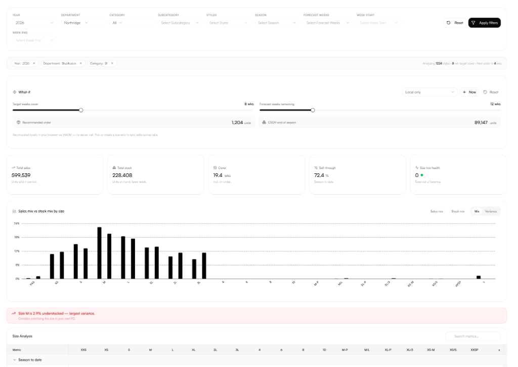
Watching it in-season, sales mix against stock mix, is the same lens applied after the buy lands. Compare how sizes are selling to how stock is held, and the imbalances show up as variance:
| Size | Sales mix | Stock mix | Variance | Read |
|---|---|---|---|---|
| M | 30% | 22% | -8% | Under-stocked: prioritise replenishment |
| L | 25% | 20% | -5% | Under-stocked: replenish |
| XL | 12% | 8% | -4% | Under-stocked: replenish |
| S | 20% | 20% | 0% | Balanced |
| XS | 8% | 16% | +8% | Over-stocked: hold or mark down |
| XXL | 5% | 14% | +9% | Over-stocked: hold or mark down |
A negative variance means demand is outrunning stock and a size is about to break; a positive variance means stock is trapped. Reading this weekly, by store grade, is how you catch a breaking size while there is still time to move stock, not after it has already cost the sale.
Method
Seven steps to a curve that holds.
- Start from clean sales history.
- Use full-price periods when the product was in stock in all sizes. Learning from data that includes stockouts teaches you the wrong curve (see "where it breaks").
- Segment the curve.
- Build separate curves by product type, store grade, climate or region, and channel, since a single national curve hides real differences.
- Calculate the size percentages.
- Convert the clean history into a demand share per size for each segment.
- Apply it to the buy.
- Size the purchase order to the curve rather than a flat ratio.
- Apply it to allocation.
- Send each store the size mix its grade actually demands, not an even spread.
- Replenish back to the curve.
- Top up stores so the on-hand size mix stays aligned to demand as the season trades.
- Refresh with recent trade.
- Re-cut the curve as new, clean sales data comes in so it tracks shifting demand.
The right size split, every store, every week.
Size your buy, allocation and replenishment to real demand, by store grade, in one place.
Where it breaks
Size curves go wrong in five ways.
- Flat or habitual buying.
- Splitting the buy evenly, or reusing an old ratio, ignores that demand is uneven and shifts over time.
- The stockout death spiral.
- If you build next season's curve from sales history that includes stockouts, a size that was unavailable looks like it did not sell, so you buy even less of it and break it again. Clean the history first.
- One national curve.
- A single curve applied to every store ignores size differences by region, climate and store grade, over-stocking some stores and starving others.
- No in-season monitoring.
- Without watching sales mix against stock mix, breaking sizes go unnoticed until the option has already lost its run.
- Size data stuck in spreadsheets.
- When the curve lives in a spreadsheet disconnected from allocation and replenishment, the insight never reaches the stock decision it should drive.
In merchmix
In merchmix, curves are applied by store grade.
merchmix includes a dedicated size-curve workspace, assortment size analysis and size curve planning. It compares sales mix against stock mix and projects size-level closing stock on hand (CSOH) across the season, surfacing size-curve gaps, trapped stock and sizing opportunities before they turn into lost sales or markdown.
Because merchmix runs on store grades, demand curves are applied by grade, so climate, footfall and location differences are built into the size mix each store receives, rather than a single national curve. That size intelligence feeds directly into core plus, where allocation and replenishment are driven by grade, so decisions move by size and by week against real demand instead of assumptions.
- What is assortment planning?
- Breadth, depth and store clusters. Read the guide
- What is a WSSI?
- How the weekly WSSI (MFP) plan tracks stock and intake. Read the guide
- Allocation and replenishment
- How stock reaches each store by grade. Read the guide
Questions, answered.
What is a size curve?
A size curve is the distribution of demand across the sizes within a product or category (for example XS 8%, S 20%, M 30%, L 25%, XL 12%, XXL 5%). It tells you what share of units each size should represent, based on real customer demand rather than an even split.
What is size curve optimization?
Size curve optimization is the practice of buying, allocating and replenishing stock in the size proportions that match real demand, so core sizes stay in stock and tail sizes do not build up into markdown. It applies the size curve to the buy, the store allocation and weekly replenishment.
What is the difference between sales mix and stock mix?
Sales mix is how units are actually selling across sizes right now; stock mix is how current stock is distributed across sizes. When they diverge (stock heavy in slow sizes, thin in fast ones) you have a size imbalance that is costing full-price sales at one end and creating markdown at the other.
What is a broken size or size gap?
A broken size is a size that has sold out mid-season. Because a shopper who cannot find their size often buys nothing rather than sizing up or down, a broken size suppresses sell-through across the whole option, not just that one size, which is why keeping core sizes in stock matters more than the size-level revenue alone suggests.
Why shouldn't you build size curves from raw sales history?
Because raw history includes periods when sizes were out of stock. A size that was unavailable records low sales, so if you learn the curve from that data you buy even less of it next time and break it again, leading to a stockout death spiral. Build curves from clean, full-price, in-stock periods instead.
Should size curves vary by store?
Yes. Demand by size differs by region, climate, footfall and store grade, so a single national curve over-stocks some stores and starves others. The most accurate approach applies size curves by store grade, so each store receives the size mix its customers actually demand.
How does size curve optimization relate to allocation and replenishment?
The size curve sets the target size mix; allocation sends each store that mix by grade; replenishment tops stores back up to the curve as they trade. Without an accurate curve, allocation and replenishment move the wrong sizes to the wrong stores, however good the total quantity is.
Can you manage size curves in Excel?
You can start in Excel, but it breaks down at scale: cleaning stockout bias from history, cutting curves by store grade, projecting size-level stock, and keeping the curve connected to live allocation and replenishment becomes slow and error-prone. Purpose-built size-curve planning keeps the analysis and the stock decision in one connected place.
Broken sizes cost full-price sales.
Size every buy, allocation and top-up to real demand, by grade and by week, in one connected platform.